Parallel Processing
We have mentioned that the operation of many numerical methods can be speeded up by the proper use of parallel processing or distributed systems.
- Vector/Matrix Operations:
- For inner products, a very elementary case, we assume we have two vectors,
 ,
,  , of length
  , and an equal number of parallel processors,
 , where each
  contains the components,
  .
.
- Then the multiplication of all the
 can be done in parallel in one time unit.
- if the processors are connected suitably we can actually do the addition part in
 time units.
- This assumes a high degree of connectivity between the processors. The different designs are referred to as the topologies of the systems.
- Suppose our processors were only connected as a linear array in which the communication send/receive is just between two adjacent processors.
- Then our addition of the elements would be
 time steps, because we could do an addition at each end in parallel and proceed to the middle.
- The -dimensional hypercube is a graph with
 vertices in which each vertex has edges (is connected to other vertices). This graph can be easily defined recursively because there is an easy albalgorithm determine the order in which the vertices are connected. See Fig. 1.
Figure 1:
Connectivity between the processors (topologies).
|
|
- Two vertices are adjacent if and only if the indices differ in exactly one bit.
- We can get to the
 -dimensional hypercube by making two copies of the -dimensional hypercube and then adding a zero to the leftmost bit of the first -dimensional cube and then doing the same with a l to the second cube.
- There are many other designs for connecting the processors. Such designs include names like star, ring, torus, mesh
- For the matrix/vector product, Ax, we assume that processor contains the
 th row of
  as well as the vector,
  .
.
- Because one processor is performing this dot product of row of and of vector , the whole operation will only take
 units of time.
- For the matrix/matrix product, AB, for two
 matrices, we suppose that we have
  processors. Before we start our computations each processor,
  will have received the values for row of and column
  of
of  . Based on our previous discussion, we can expect the time to be .
- Gaussian Elimination:
- Problems in Using Parallel Processors:
- The algorithm described here does not pivot. Thus, our solution may not be as numerically stable as one obtained via a sequential algorithm with partial pivoting.
- The coefficient matrix is assumed to be nonsingular. It is easy to check for singularity at each stage of the row reduction, but such error-handling will more than double the running time of the algorithm.
- We have ignored the communication and overhead time costs that are involved in parallelization. Because of these costs, it is probably more efficient to solve small systems of equation using a sequential algorithm.
- Other, perhaps faster, parallel algorithms exist for solving systems of linear equations.
- Iterative Solutions -The Jacobi Method
- Recall that at each iteration of the algorithm a new solution vector
 is computed using only the elements of the solution vector from the previous iteration,
  .
.
- Because Gauss-Seidel iteration requires that the new iterates for each variable be used after they have been obtained, this method cannot be speeded up by parallel processing.
2004-11-03
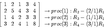
![\fbox{\parbox{11cm}{
Sequential Processing (without pivoting)\\
For j = 1 To (n...
... \\
a[i, k] = a[i, k] - a[i,j]/a[j,j]*a[j,k] \\
End For k \\
End For i \\
}}](img109.png)
![\includegraphics[scale=1]{figures/2.1.ps}](img100.png)