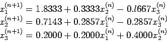
The iterative methods depend on the rearrangement of the equations in this manner:
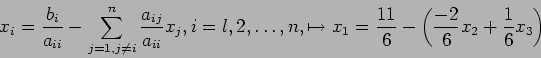
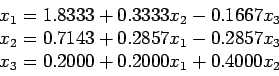
Each equation now solved for the variables in succession:
We begin with some initial approximation to the value of the variables. (Each component might be taken equal to zero if no better initial estimates are at hand.)
The new values are substituted in the right-hand sides to generate a second approximation, and the process is repeated until successive values of each of the variables are sufficiently alike.
(1)
Starting with an initial vector of
, we get
Table 2:
Successive estimates of solution (Jacobi method)
First
Second
Third
Fourth
Fifth
Sixth
Ninth
0
1.833
2.038
2.085
2.004
1.994
2.000
0
0.7l4
1.181
l.053
l.001
0.990
l.000
0
0.200
0.852
1.080
l.038
l.00l
1.000
Note that this method is exactly the same as the method of fixed-point iteration for a single equation that was discussed in Section , but it is now applied to a set of equations; we see this if we write Eq. 1 in the form of
which is identical to
as used in Section .
In the present context, and refer to the th and st iterates of a vector rather than a simple variable, and is a linear transformation rather than a nonlinear function.
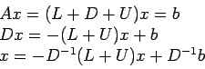
Now, let , where
rewritten as
From this we have, identifying on the left as the new iterate,
The procedure we have just described is known as the Jacobi method, also called ''the method of simultaneous displacements'', because each of the equations is simultaneously changed by using the most recent set of -values. See Table 2.
![\begin{displaymath}
Ax=b,
\left[
\begin{array}{rrr}
6 &-2 & 1 \\
-2 & 7 & 2 \...
...left[
\begin{array}{r}
11\\
5\\
-1\\
\end{array}\right]
\end{displaymath}](img78.png)
![\begin{displaymath}
L=\left[
\begin{array}{rrr}
0 & 0 & 0 \\
-2 & 0 & 0 \\
...
...&-2 & 1 \\
0 & 0 & 2 \\
0 & 0 & 0 \\
\end{array} \right]
\end{displaymath}](img80.png)
![\begin{displaymath}
b'=D^{-1}b=\left[
\begin{array}{l}
1.8333 \\
0.7143 \\
0.2000 \\
\end{array} \right]
\end{displaymath}](img84.png)
![\begin{displaymath}
D^{-1}(L + U)=\left[
\begin{array}{rrr}
0 &-0.3333 & 0.1667...
... 0 & 0.2857 \\
-0.2000 & -0.4000 & 0 \\
\end{array} \right]
\end{displaymath}](img85.png)