Next: Economizing a Power Series Up: Chebyshev Polynomials and Chebyshev Previous: Chebyshev Polynomials and Chebyshev
function T=Tch(n)
if n==0
disp('1')
elseif n==1
disp('x')
else
t0='1';
t1='x';
for i=2:n
T=symop('2*x','*',t1,'-',t0);
t0=t1;
t1=T;
end
end
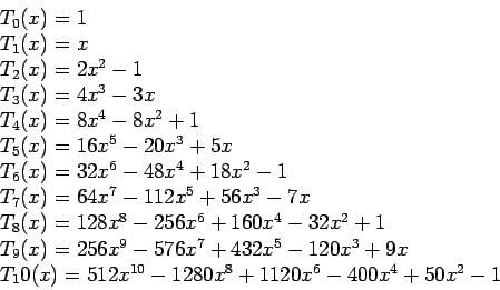
>>Tch(5)
>>collect(ans)
ans= 16*x^5-20*x^3+5*x
![\includegraphics[scale=1.2]{figures/4.1.ps}](img29.png)