The following function is given
This nonlinear equation ( ) is solved by using four methods, namely Bisection, Regula Falsi, Newton's, Muller's methods. See the following MATLAB commands;
>> f = inline ( ' 3*sin( x) - exp ( x)/4 -1');
>> df = inline ( ' 3*cos( x) - exp ( x)/4');
>> fplot(f,[-7 -3]); grid on;
>> format short e
>> bisect(f,-7,-5,fzero(f,[-7 -5]),1e-5);
>> regula(f,-7,-5,fzero(f,[-7 -5]),1e-5,eps,20);
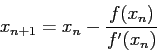
>> newton(f,df,-7,fzero(f,[-7 -5]),1e-5,eps,20);
>> muller(f,-7,-6,-5,fzero(f,[-7 -5]),1e-5,eps,20);
Plot of the function is given at the following figure;
Then, the following tables are obtained.
Table:
Obtained root values at each iteration for all of four methods.
| iteration |
Bisection |
Regula |
Newton |
Muller |
| 1 |
-6.0000e+00 |
-5.5672e+00 |
-5.4650e+00 |
-5.7134e+00 |
| 2 |
5.5000e+00 |
-5.7373e+00 |
-5.8008e+00 |
-5.7604e+00 |
| 3 |
-5.7500e+00 |
-5.7575e+00 |
-5.7596e+00 |
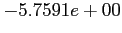
-5.7591e+00 |
| 4 |
-5.8750e+00 |
-5.7590e+00 |
-5.7591e+00 |
-5.7591e+00 |
| 5 |
-5.8125e+00 |
-5.7591e+00 |
-5.7591e+00 |
- |
| 6 |
-5.7812e+00 |
-5.7591e+00 |
- |
- |
Table:
Obtained function values at each iteration for all of four methods.
| iteration |
Bisection |
Regula |
Newton |
Muller |
| 1 |
-4.4179e-01 |
3.1174e-01 |
4.5882e-01 |
7.8084e-02 |
| 2 |
4.1006e-01 |
3.7524e-02 |
-7.3051e-02 |
-2.2184e-03 |
| 3 |
1.5762e-02 |
2.8928e-03 |
-8.1042e-04 |
4.1882e-06 |
| 4 |
-2.0681e-01 |
2.0926e-04 |
-1.0968e-07 |
-4.0674e-11 |
| 5 |
-9.3753e-02 |
1.5061e-05 |
-2.2204e-15 |
- |
| 6 |
-3.8525e-02 |
1.0836e-06 |
- |
- |
- i
- Analyze these tables. Is the convergence sustained for the each methods? For the sustained ones; at which iteration and why?
- ii
- If the exact value is given as
 , fill the following table for two methods. Choose two methods and use scientific notation with five significant figures.;
|
iteration |
 |
 |
 |
 |
|
1 |
-2.4087e-01 |
1.9191e-01 |
2.9418e-01 |
4.5735e-02 |
|
2 |
2.5913e-01 |
2.1820e-02 |
-4.1715e-02 |
-1.2812e-03 |
|
3 |
9.1313e-03 |
1.6722e-03 |
-4.6817e-04 |
2.4198e-06 |
|
4 |
-1.1587e-01 |
1.2090e-04 |
-6.3367e-08 |
-2.3500e-11 |
|
5 |
-5.3369e-02 |
8.7017e-06 |
-1.7764e-15 |
- |
|
6 |
-2.2119e-02 |
6.2607e-07 |
- |
|
|
iteration |
 |
 |
 |
 |
|
1 |
-2.4087e-01 |
1.9191e-01 |
2.9418e-01 |
4.5735e-02 |
|
2 |
-1.0758e+00 |
1.1370e-01 |
-1.4180e-01 |
-2.8014e-02 |
|
3 |
3.5238e-02 |
7.6636e-02 |
1.1223e-02 |
-1.8887e-03 |
|
4 |
-1.2689e+01 |
7.2305e-02 |
1.3535e-04 |
-9.7116e-06 |
|
5 |
4.6060e-01 |
7.1972e-02 |
2.8033e-08 |
- |
|
6 |
4.1445e-01 |
7.1948e-02 |
- |
- |
- iii
- What can you say about the speed of convergences for each method?
- iv
- Which method is the best one? Why?
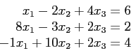
Consider the linear system;
- viii
- Solve this system by Gaussian elimination with pivoting. How many row interchanges are needed?
- ix
- What is the value of determinant?
- x
- Obtain the
 decomposition of the system.
- xi
- Repeat without any row interchanges (only for the first item). Do you get the same results? Why?
>> A=[1 -2 4; 8 -3 2; -1 10 2]
>> b=[6 2 4]
>> GEPivShow(A,b')
Begin forward elimination with Augmented system:
     1    -2     4     6
     8    -3     2     2
    -1    10     2     4
Swap rows 1 and 2;  new pivot = 8
After elimination in column 1 with pivot = 8.000000
    8.0000   -3.0000    2.0000    2.0000
         0   -1.6250    3.7500    5.7500
         0    9.6250    2.2500    4.2500
Swap rows 2 and 3;  new pivot = 9.625
After elimination in column 2 with pivot = 9.625000
    8.0000   -3.0000    2.0000    2.0000
         0    9.6250    2.2500    4.2500
         0         0    4.1299    6.4675
ans =   -0.1132     0.0755     1.5660 %these are x1, x2, x3
>> det(A)
ans =   318
>> 8.0000*9.6250 *4.1299 %product of the diagonal of U
ans =  318.0023
% For LU-decomposition
>> [L,U,pv] = luPiv(A)
L =    1.0000         0         0
        -0.1250    1.0000         0
         0.1250   -0.1688    1.0000
U =   8.0000   -3.0000    2.0000
         0    9.6250    2.2500
         0         0    4.1299
pv =

     2
     3
     1
% two times pivoting
% solution is completed
%**********************************************
% For proving purpose
>> A=[1 -2 4; 8 -3 2; -1 10 2]
A =
     1    -2     4
     8    -3     2
    -1    10     2
% our Idendity matrix becomes for swaping rows 1 and 2
>> pivoting1=[0 1 0; 1 0 0; 0 0 1]
pivoting1 =
     0     1     0
     1     0     0
     0     0     1
% apply this pivoting to our original matrix
>> A=pivoting1*A
A =
     8    -3     2
     1    -2     4
    -1    10     2
% our Idendity matrix becomes for swaping rows 2 and 3
>> pivoting2=[1 0 0; 0 0 1; 0 1 0]
pivoting2 =
     1     0     0
     0     0     1
     0     1     0

% also apply this pivoting to our pivoted matrix
>> A=pivoting2*A
A =
     8    -3     2
    -1    10     2
     1    -2     4
>> [L,U,pv] = luPiv(A)
L =
   1.000000000000000                   0                   0
  -0.125000000000000   1.000000000000000                   0
   0.125000000000000  -0.168831168831169   1.000000000000000
U =
   8.000000000000000  -3.000000000000000   2.000000000000000
                   0   9.625000000000000   2.250000000000000
                   0                   0   4.129870129870130
pv =
     1
     2
     3
% it is proved.
%**********************************************
% for not pivoting case;
>> GEshow(A,b')
Begin forward elimination with Augmented system:
     1    -2     4     6
     8    -3     2     2
    -1    10     2     4
After elimination in column 1 with pivot = 1.000000
     1    -2     4     6
     0    13   -30   -46
     0     8     6    10
After elimination in column 2 with pivot = 13.000000
    1.0000   -2.0000    4.0000    6.0000
         0   13.0000  -30.0000  -46.0000
         0         0   24.4615   38.3077
ans =    -0.1132     0.0755    1.5660
>> 1.0000*13.0000*24.4615
ans =   317.9995
% Solutions are the same. They are same because the system is
% not ill-conditioned.
![\includegraphics[scale=0.6]{figures/28}](img5.png)
![\includegraphics[scale=0.5]{figures/30}](img30.png)