Ceng 375 Numerical Computing
Final
Jan 18, 2012 10.00-11.50
Good Luck!
- (10 pts) An engineer runs the same FORTRAN program on two different computers, a PC and a UNIX Workstation. Neither system produces any error messages, but the resulting outputs differ by several orders of magnitude more than machine precision. What, if any, reasonable explanations are there for this phenomenon?
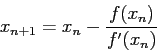
- (25 pts) In Newton's method the approximation
 to a root of
  is computed from the approximation
  using the equation
- i
- (10 pts) Derive the above formula, using a Taylor series of
 .
.
- ii
- (15 pts) For
 , refine the approximation
  to the unique root of by carrying out one iteration of Newton's method.
- Choose only three questions. Each question is 25 points. Circle/Mark the question number that you want to be graded.
- 1
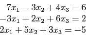
- Consider the linear system
- iii
- (10 pts) Solve this system with the Jacobi method. First rearrange to make it diagonally dominant if possible. Use
![$[0,0,0]$](img9.png) as the starting vector.
as the starting vector.
- iv
- (15 pts) Repeat with Gauss-Seidel method. Compare with Jacobi method.
- 2
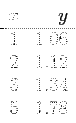
- For the given data points;
- v
- (15 pts) construct the divided-difference table.
- vi
- (5 pts) interpolate for
 .
.
- vii
- (5 pts) extrapolate for
 .
.
- 3
- Least Squares Method
- viii
- (12.5 pts) A function
 is to be used as an approximation to a set of data
  with
with
 . Suppose further that the function depends on two parameters
  and
and  . Provide full details of how the parameters and can be determined.
- ix
- (12.5 pts) Using the result of the previous item, obtain the normal equations for the function
 . Do not attempt to solve these equations.
- 4
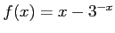
- Write the expression to economize the the Maclaurin series for
 with the precision 0.008 by using Chebyshev polynomials. Do not perform the calculations.
- 5
- Consider the following table of data
 |
 |
| 0.0000 |
0.0000 |
| 0.2000 |
0.5879 |
| 0.4000 |
1.0637 |
| 0.6000 |
1.3927 |
| 0.8000 |
1.5573 |
| 1.0000 |
1.5575 |
| 1.2000 |
1.4091 |
- x
- (7.5 pts) Approximate
 dx using the Trapezoidal Rule and a step size of
  .
.
- xi
- (7.5 pts) Approximate
dx using the Trapezoidal Rule and a step size of
 .
.
- xii
- (10 pts) Estimate the error in your answer to previous item.
Hint: Use the procedure to estimate the proportionality factor,  .
.

Cem Ozdogan
2012-01-22