- The procedure just described has a major problem.
- While it may be satisfactory for hand computations with small systems, it is inadequate for a large system.
- Observe that the transformed coefficients can become very large (getting bigger!) as we convert to a triangular system.
- The method that is called Gaussian elimination avoids this by subtracting
 times the first
equation from the
times the first
equation from the  equation to make the transformed numbers in the first column equal to zero.
- We do similarly for the rest of the columns.
- Observe that zeros may be created in the diagonal positions even if they are not present in the original matrix of coefficients.
- A useful strategy to avoid (if possible) such zero divisors is to rearrange the equations so as to put the coefficient of largest magnitude on the diagonal at each step.
- This is called pivoting.
- Repeat the example of the previous section,
- The method we have just illustrated is called Gaussian elimination.
- In this example, no pivoting was required to make the largest coefficients be on the diagonal.
- Back-substitution, gives us
Example m-file: Show steps in Gauss elimination and back substitution. No pivoting. (http://siber.cankaya.edu.tr/ozdogan/NumericalComputations/mfiles/chapter2/GEshow.m GEshow.m)
- We shall obtain answers that are just close approximations to the exact answer because of round-off error.
- When there are many equations, the effects of round-off (the term is applied to the error due to chopping as well as when rounding is used) may cause large effects.
- In certain cases, the coefficients are such that the results are particularly sensitive to round off; such systems are called ill-conditioned.
- if we had stored the ratio of coefficients in place of zero (we show these in parentheses), our final form would have been
- The original matrix can be written as the product:
- This procedure is called a
 -decomposition of
  .
.
- In this case,
where  is lower-triangular and
  is upper-triangular.
- The determinant of two matrices,
 , is the product of each of the determinants, for this example we have
Because is triangular and has only ones on its diagonal so that  .
.
- Thus, for our example, we have
since is upper-triangular and its determinant is just the product of the diagonal elements.
- When there are row interchanges
where the exponent m represents the number of row interchanges.
- Example. Solve the following system of equations using Gaussian elimination.
- In addition, obtain the determinant of the coefficient matrix and the decomposition of this matrix.
- The augmented coefficient matrix is
- We cannot permit a zero in the
 position because that element is the pivot in reducing the first column.
- We could interchange the first row with any of the other rows to avoid a zero divisor, but interchanging the first and fourth rows is our best choice. This gives
- 4
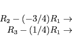
- We again interchange before reducing the second column, not because we have a zero divisor, but because we want to preserve accuracy. Interchanging the second and third rows puts the element of largest magnitude on the diagonal.
- 5
- Now we reduce in the second column
- 6
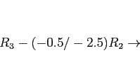
- No interchange is indicated in the third column. Reducing, we get
- 7
- Back-substitution gives
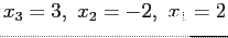
- The correct (exact) answers are
 .
.
- In this calculation we have carried five significant figures and rounded each calculation.
- Even so, we do not have five-digit accuracy in the answers.
- The discrepancy is due to round off.
- Example m-files: (http://siber.cankaya.edu.tr/ozdogan/NumericalComputations/mfiles/chapter2/GEshow.m GEshow.m, http://siber.cankaya.edu.tr/ozdogan/NumericalComputations/mfiles/chapter2/GEPivShow.m GEPivShow.m)
- In this example, if we had replaced the zeros below the main diagonal with the ratio of coefficients at each step, the resulting augmented matrix would be
- This gives a LU decomposition as
- It should be noted that the product of these matrices produces a permutation of the original matrix, call it
 , where
- The determinant of the original matrix of coefficients can be easily computed according to the formula
which is close to the exact solution: -234.
- The exponent 2 is required, because there were two row interchanges in solving this system.
- To summarize
- The solution to the four equations
- The determinant of the coefficient matrix
- A decomposition of the matrix, , which is just the original matrix, , after we have interchanged its rows.
- ``These'' are readily obtained after solving the system by Gaussian elimination method.
Example m-file: LU factorization without pivoting. (http://siber.cankaya.edu.tr/ozdogan/NumericalComputations/mfiles/chapter2/luNopiv.m luNopiv.m)
Example m-file: LU factorization with partial pivoting. (http://siber.cankaya.edu.tr/ozdogan/NumericalComputations/mfiles/chapter2/luPiv.m luPiv.m)
Cem Ozdogan
2011-12-27
![\begin{displaymath}
\left[
\begin{array}{rrrr}
4 & -2 & 1 &15 \\
-3 & -1 & 4 &8 \\
1 & -1 & 3 &13 \\
\end{array} \right],
\end{displaymath}](img456.png)
![\begin{displaymath}
\left[
\begin{array}{rrrr}
4 & -2 & 1 &15 \\
0 & -2.5 & 4.75 &19.25 \\
0 & -0.5 & 2.75 & 9.25 \\
\end{array} \right],
\end{displaymath}](img465.png)
![\begin{displaymath}
\left[
\begin{array}{rrrr}
4 & -2 & 1 &15 \\
0 & -2.5 & 4.75 & 19.25 \\
0 & 0 & 1.8 & 5.40 \\
\end{array} \right]
\end{displaymath}](img467.png)
![\begin{displaymath}
\left[
\begin{array}{rrrr}
4 & -2 & 1 &15 \\
(-0.75) & -2...
...9.25 \\
(0.25) & (0.20) & 1.8 & 5.40 \\
\end{array} \right]
\end{displaymath}](img470.png)
![\begin{displaymath}
\underbrace{\left[
\begin{array}{rrr}
1 & 0 & 0 \\
-0.75 & 1 & 0 \\
0.25 & 0.20 & 1 \\
\end{array} \right]}_L*
\end{displaymath}](img472.png)
![\begin{displaymath}
\underbrace{\left[
\begin{array}{rrr}
4 & -2 & 1 \\
0 & -2.5 & 4.75 \\
0 & 0 & 1.8 \\
\end{array} \right]}_U
\end{displaymath}](img473.png)
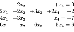
![\begin{displaymath}
\left[
\begin{array}{rrrrr}
0 & 2 & 0 & 1 &0 \\
2 & 2 & 3...
...& -3 & 0 & 1 &-7 \\
6 & 1 &-6 &-5 &6 \\
\end{array} \right]
\end{displaymath}](img484.png)
![\begin{displaymath}
\left[
\begin{array}{rrrrr}
6 & 1 &-6 &-5 &6 \\
2 & 2 & 3...
...& -3 & 0 & 1 &-7 \\
0 & 2 & 0 & 1 &0 \\
\end{array} \right]
\end{displaymath}](img486.png)
![\begin{displaymath}
\left[
\begin{array}{rrrrr}
6 & 1 &-6 &-5 &6 \\
0 &1.6667...
... & 4 &4.3333&-11 \\
0 & 2 & 0 & 1 &0 \\
\end{array} \right]
\end{displaymath}](img487.png)
![\begin{displaymath}
\left[
\begin{array}{rrrrr}
6 & 1 &-6 &-5 &6 \\
0 &-3.666...
...67& 5 &3.6667&-4 \\
0 & 2 & 0 & 1 &0 \\
\end{array} \right]
\end{displaymath}](img488.png)
![\begin{displaymath}
\left[
\begin{array}{rrrrr}
6 & 1 &-6 &-5 &6 \\
0 &-3.666...
...1\\
0 & 0 & 2.1818 & 3.3636 &-5.9999 \\
\end{array} \right]
\end{displaymath}](img489.png)
![\begin{displaymath}
\left[
\begin{array}{rrrrr}
6 & 1 &-6 &-5 &6 \\
0 &-3.666...
...9.0001\\
0 & 0 & 0 & 1.5600 &-3.1199 \\
\end{array} \right]
\end{displaymath}](img490.png)
![\begin{displaymath}
\left[
\begin{array}{rrrrr}
6 & 1 &-6 &-5 &6 \\
(0.66667)...
... (-0.54545) & (0.32) & 1.5600 &-3.1199 \\
\end{array} \right]
\end{displaymath}](img494.png)
![\begin{displaymath}
\left[
\begin{array}{rrrrr}
1&0&0&0\\
0.66667 & 1 & 0 & 0...
... & 1 &0 \\
0.0 & -0.54545 & 0.32 & 1 \\
\end{array} \right]
\end{displaymath}](img495.png)
![\begin{displaymath}
\left[
\begin{array}{rrrr}
6 & 1 &-6 &-5 \\
0&-3.6667 & ...
... & 6.8182 &5.6364\\
0& 0 &0 & 1.5600 \\
\end{array} \right]
\end{displaymath}](img496.png)
![\begin{displaymath}
A'=\left[
\begin{array}{rrrr}
6 & 1 &-6 &-5 \\
4 & -3 & 0...
... \\
2 & 2 & 3 & 2 \\
0 & 2 & 0 & 1 \\
\end{array} \right]
\end{displaymath}](img498.png)
![\includegraphics[scale=1.5]{figures/2-2}](img469.png)
![\includegraphics[scale=1.5]{figures/2-3}](img493.png)
![\includegraphics[scale=1.5]{figures/2-4}](img500.png)