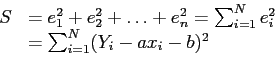
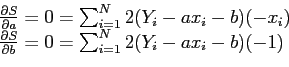
Least-Squares Approximations

• Until now, we have assumed that the data are accurate,
• but when these values are derived from an experiment, there is some error in the measurements.

Figure 5.6: Resistance vs Temperature graph for the Least-Squares Approximation.

• Some students are assigned to find the effect of temperature on the resistance of a metal wire.
• They have recorded the temperature and resistance values in a table and have plotted their findings, as seen in Fig. 5.6.
• The graph suggest a linear relationship.
  $$R=aT + b$$

• Values for the parameters, $a$ and $b$, can be obtained from the plot.

• If someone else were given the data and asked to draw the line,
• it is not likely that they would draw exactly the same line and they would get different values for $a$ and $b$.
• In analyzing the data, we will assume that the temperature values are accurate
• and that the errors are only in the resistance numbers; we then will use the vertical distances.

• A way of fitting a line to experimental data that is to minimize the deviations of the points from the line.
• The usual method for doing this is called the least-squares method.
• The deviations are determined by the distances between the points and the line.

  Figure 5.7: Minimizing the deviations by making the sum a minimum.

  
  • Consider the case of only two points (See Fig. 5.7).
  • Obviously, the best line passes through each point,
  • but any line that passes through the midpoint of the segment connecting them has a sum of errors equal to zero.

• We might first suppose we could minimize the deviations by making their sum a minimum, but this is not an adequate criterion.
• We might accept the criterion that we make the magnitude of the maximum error a minimum (the so-called minimax criterion).
• The usual criterion is to minimize the sum of the squares of the errors, the least-squares principle.
• In addition to giving a unique result for a given set of data, the least-squares method is also in accord with the maximum-likelihood principle of statistics.
• If the measurement errors have a so-called normal distribution
• and if the standard deviation is constant for all the data,
• the line determined by minimizing the sum of squares can be shown to have values of slope and intercept that have maximum likelihood of occurrence.

• Let $Y_i$ represent an experimental value, and let $y_i$ be a value from the equation
  $$y_i=ax_i + b$$
  where $x_i$ is a particular value of the variable assumed to be free of error.
• We wish to determine the best values for $a$ and $b$ so that the $y$'s predict the function values that correspond to $x$-values.
• Let
  $$e_i= Y_i-y_i$$

• The least-squares criterion requires that $S$ be a minimum.
  $$\begin{array}{ll} S & =e_1^2+e_2^2+\ldots+e_n^2=\sum_{i=1}^N e_i^2 \\ & =\sum_{i=1}^N (Y_i-ax_i-b)^2 \\ \end{array}$$

• $N$ is the number of $(x,Y)$-pairs.

• We reach the minimum by proper choice of the parameters $a$ and $b$, so they are the variables of the problem.
• At a minimum for $S$, the two partial derivatives will be zero.
  $$\partial S/\partial a        \&       \partial S/\partial b$$

• Remembering that the $x_i$ and $Y_i$ are data points unaffected by our choice our values for $a$ and $b$, we have
  $$\begin{array}{l} \frac{\partial S}{\partial a}=0= \sum_{i=1... ...}{\partial b}=0= \sum_{i=1}^N 2(Y_i-ax_i-b)(-1) \\ \end{array}$$

• Dividing each of these equations by $-2$ and expanding the summation, we get the so-called normal equations
  $$\begin{array}{rl} a\sum x_i^2+b\sum x_i & =\sum x_iY_i\\ a\sum x_i+bN & =\sum Y_i\\ \end{array}$$

• All the summations are from $i= 1$ to $i= N$.

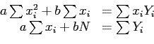
• Solving these equations simultaneously gives the values for slope and intercept $a$ and $b$.
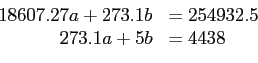
• For the data in Fig. 5.6 we find that
  $$N= 5,\sum T_i=273.1,\sum T_i^2=18607.27,$$
  $$\sum R_i= 4438,\sum T_iR_i = 254932.5$$

• Our normal equations are then
  $$\begin{array}{rl} 18607.27 a + 273.1 b& =254932.5\\ 273.1a + 5b &=4438\\ \end{array}$$

• From these we find $a = 3.395$, $b= 702.2$, and
  $$R=702.2+3.395T$$

• MATLAB gets a least-squares polynomial with its polyfit command.
• When the numbers of points (the size of $x$) is greater than the degree plus one, the polynomial is the least squares fit.