Hands-on-Interpolation and Curve Fitting with MATLAB II

1. For the given data points;
   
   $$\begin{array}{rr} x & y \\ \hline 2 & 2.12 \\ 4 & 2.24 \\ 6 & 2.68 \\ 10 & 3.56 \\ \end{array}$$
   
   

   i

   construct the divided-difference table by hand

   ii

   run the MATLAB code (http://siber.cankaya.edu.tr/ozdogan/NumericalComputations/mfiles/chapter3/newpoly.m newpoly.m) and compare with your table.

   • interpolate for $x=8$
   • extrapolate for $x=11$

   iii

   run the MATLAB code (http://siber.cankaya.edu.tr/ozdogan/NumericalComputations/mfiles/chapter3/divDiffTable.m divDiffTable.m)

   • interpolate for $x=8$
   • extrapolate for $x=11$

   Hint: Open these m-files with the editor. Then execute the codes according to the first line. Use these outputs to inter/extrapolate (see lecture notes).

2. The MATLAB procedure for polynomial least-squares is polyfit. Study the following example;

   
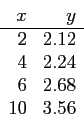
3. For the given data points;
   

   T ($^\circ C$)	R (ohms)
   20.5	765
   32.7	826
   51.0	873
   73.2	942
   95.7	1032

   iv

   Plot it (such as plot(x,Y,'o')).

   v

   The graph suggest a linear relationship.
   

   $$y=ax + b$$

   
   

   values for the parameters, $a$ and $b$, can be obtained from the plot.

   vi

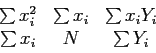
   Write a MATLAB code that calculates each summation;
   

   $$\begin{array}{ccc} \sum x_i^2 & \sum x_i & \sum x_iY_i\\ \sum x_i & N & \sum Y_i\\ \end{array}$$

   
   

   All the summations are from $i= 1$ to $i= N$.

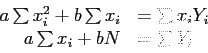
   vii

   Then it is obtained as
   

   $$\begin{array}{rl} a\sum x_i^2+b\sum x_i & =\sum x_iY_i\\ a\sum x_i+bN & =\sum Y_i\\ \end{array}$$

   
   

   Solving these equations simultaneously gives the values for slope and intercept $a$ and $b$. Now, we have a function in the form;
   

   $$y=ax + b$$

   
   

   viii

   Plot them (such as plot(x,y,x,Y,'o')).