Next: Use of Orthogonal Polynomials Up: week9 Previous: Nonlinear Data, Curve Fitting
![\begin{displaymath}
A=\left[
\begin{array}{rrrrr}
1 & 1 & 1 & 1 & 1 \\
x_1 & ...
... x_1^n & x_2^n & x_3^n & \ldots & x_N^n\\
\end{array} \right]
\end{displaymath}](img37.png)
![$\displaystyle \overbrace{\left[
\begin{array}{rrrrr}
1 & 1 & 1 & 1 & 1 \\
x...
...Y_i\\
\sum x_i^2Y_i\\
\vdots \\
\sum x_i^n Y_i\\
\end{array} \right]$](img41.png) |
(4) |
![\begin{displaymath}
\overbrace{\left[
\begin{array}{rrrrr}
1 & 1 & 1 & \ldots &...
...^n & x_2^n & x_3^n & \ldots & x_N^n\\
\end{array} \right]}^A*
\end{displaymath}](img45.png)
![\begin{displaymath}
\overbrace{\left[
\begin{array}{rrrrr}
1 & x_1 & x_1^2 & \l...
...& x_N & x_N^2 & \ldots & x_N^n \\
\end{array} \right]}^{A^T}=
\end{displaymath}](img46.png)
![\begin{displaymath}
\underbrace{\left[
\begin{array}{rrrrrl}
N & \sum x_i & \sum...
... x_i^{n+3} & \ldots & \sum x_i^{2n}\\
\end{array} \right]}_B
\end{displaymath}](img47.png)
![\begin{displaymath}
\overbrace{\left[
\begin{array}{rrrrr}
1 & x_1 & x_1^2 & \l...
...& x_N & x_N^2 & \ldots & x_N^n \\
\end{array} \right]}^{A^T}*
\end{displaymath}](img49.png)
![\begin{displaymath}
\overbrace{\left[
\begin{array}{r}
a_0\\
a_1\\
a_2\\
\ldots\\
a_n\\
\end{array} \right]}^{a}=
\end{displaymath}](img50.png)
![\begin{displaymath}
\overbrace{\left[
\begin{array}{r}
y_1\\
y_2\\
y_3\\
\ldots\\
y_N\\
\end{array} \right]}^{y}
\end{displaymath}](img51.png)
R/C: 0.73, 0.78, 0.81, 0.86, 0.875, 0.89, 0.95, 1.02, 1.03, 1.055, 1.135, 1.14, 1.245, 1.32, 1.385, 1.43, 1.445, 1.535, 1.57, 1.63, 1.755.
![]() : 0.0788, 0.0788, 0.064, 0.0788, 0.0681, 0.0703, 0.0703, 0.0681, 0.0681, 0.079, 0.0575, 0.0681, 0.0575, 0.0511, 0.0575, 0.049, 0.0532, 0.0511, 0.049, 0.0532,0.0426.
: 0.0788, 0.0788, 0.064, 0.0788, 0.0681, 0.0703, 0.0703, 0.0681, 0.0681, 0.079, 0.0575, 0.0681, 0.0575, 0.0511, 0.0575, 0.049, 0.0532, 0.0511, 0.049, 0.0532,0.0426.
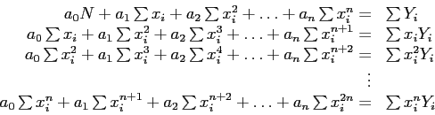
![$\displaystyle \overbrace{\left[
\begin{array}{rrrrrl}
N & \sum x_i & \sum x_i^2...
...Y_i\\
\sum x_i^2Y_i\\
\vdots \\
\sum x_i^n Y_i\\
\end{array} \right]$](img34.png)
![\begin{table}\begin{center}
\includegraphics[scale=0.3]{figures/3-15}
\end{center}
\end{table}](img54.png)
![\includegraphics[scale=0.4]{figures/3-13}](img61.png)
![\includegraphics[scale=0.4]{figures/3-16}](img71.png)