Chebyshev Series
- By rearranging the Chebyshev polynomials, we can express powers of
 in terms of them:
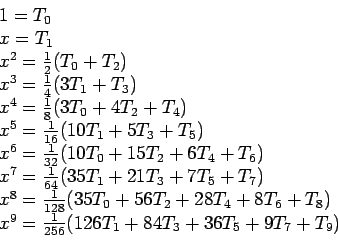 |
(6.2) |
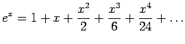
- By substituting these identities into an infinite Taylor series and collecting terms in
 , we create a Chebyshev series. For example, we can get the first four terms of a Chebyshev series by starting with the Maclaurin expansion for
  . Such a series converges more
rapidly than does a Taylor series on
. Such a series converges more
rapidly than does a Taylor series on ![$ [-1, 1]$](img820.png) ;
Replacing terms by Eqn. 6.2, but omitting polynomials beyond
;
Replacing terms by Eqn. 6.2, but omitting polynomials beyond  because we want only four terms (The number of terms that are employed determines the accuracy of the computed values), we have;
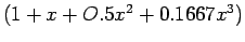
To compare the Chebyshev expansion with the Maclaurin series, we convert back to powers of , using Eqn. 6.1:
because we want only four terms (The number of terms that are employed determines the accuracy of the computed values), we have;
To compare the Chebyshev expansion with the Maclaurin series, we convert back to powers of , using Eqn. 6.1:
 |
(6.3) |
- Table 6.2 and Figure 6.2 compare the error of the Chebyshev expansion, Eqn. 6.3, with the Maclaurin series
 , using terms through
  in each case.
- The errors can be considered to be distributed more or less uniformly throughout the interval.
- In contrast to this, the Maclaurin expansion, which gives very small errors near the origin, allows the error to bunch up at the ends of the interval.
Table 6.2:
Comparison of Chebyshev series for with Maclaurin series.
![\begin{table}\begin{center}
\includegraphics[scale=1.1]{figures/4.3.ps}
\end{center}
\end{table}](img826.png) |
Figure 6.2:
Comparison of the error of Chebyshev series for with the error of Maclaurin series.
|
|
2004-12-28
![\includegraphics[scale=1.2]{figures/4.4.ps}](img827.png)