Hands-on- Interpolation and Curve Fitting with MATLAB I

1. For the given data points;
   
   $$\begin{array}{rr} x & y \\ \hline 1 & 1.06 \\ 2 & 1.12 \\ 3 & 1.34 \\ 5 & 1.78 \\ \end{array}$$
   
   
   • construct the interpolating cubic $P_3(x)=ax^3+bx^2+cx+d$.
     Hint: First, write the set of equations then solve it by writing/using a MATLAB program.
   • Interpolate for $x=4$
   • Extrapolate for $x=5.5$
   Solution:

   >> A=[1 1 1 1; 8 4 2 1; 27 9 3 1;125 25 5 1]
   >> B=[1.06 1.12 1.34 1.78]'
   >> X=uptrbk(A,B)
   X =
      -0.0200
       0.2000
      -0.4000
       1.2800
   >> X'*[27 9 3 1]'
   ans =    1.3400
   >> X'*A(3,1:4)'
   ans =    1.3400
   >> X'*[4^3 4^2 4 1]'
   ans =    1.6000
   >> X'*[(5.5)^3 (5.5)^2 5.5 1]'
   ans =    1.8025
   

2. We have given the following MATLAB code to evaluate the Lagrange polynomial $P(x)=\sum_{k=0}^N y_k \frac{\prod_{j\neq k}(x-x_j)}{\prod_{j\neq k}(x_k-x_j)}$ based on $N+1$ points $(x_k,y_k)$ for $k=0,1,\ldots,N$.

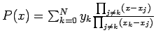
   function [C,L]=lagran(X,Y)
   %Input  - X is a vector that contains a list of abscissas
   %       - Y is a vector that contains a list of ordinates
   %Output - C is a matrix that contains the coefficents of 
   %         the Lagrange interpolatory polynomial
   %       - L is a matrix that contains the Lagrange coefficient polynomials
   
   w=length(X);
   n=w-1;
   L=zeros(w,w);
   %Form the Lagrange coefficient polynomials
   for k=1:n+1
      V=1;
      for j=1:n+1
         if k~=j
            V=conv(V,poly(X(j)))/(X(k)-X(j));
         end
      end
      L(k,:)=V;
   end
   %Determine the coefficients of the Lagrange interpolator polynomial
   C=Y*L;
   

   where
   • The poly command creates a vector whose entries are the coefficients of a polynomial with specified roots.

     >P=poly(2)
     >> 1 -2
     >>Q=poly(3)
     >> 1 -3
     

   • The conv command produces a vector whose entries are the coefficients of a polynomial that is the product of two other polynomials.

     	>>conv(P,Q)
     	>> 1 -5 6 %Thus the product of P(x) and Q(x) is x^2-5x+6
     

   Study this MATLAB code and then use the data set in the previous item to
   • interpolate for $x=4$
   • extrapolate for $x=5.5$
   Solution:
   save with the name lagran.m. Then;

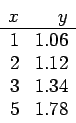
   >> X=[1 2 3 5]
   >> Y=[1.06 1.12 1.34 1.78]
   >> [C,L]=lagran(X,Y)
   C =   -0.0200    0.2000   -0.4000    1.2800
   L =
      -0.1250    1.2500   -3.8750    3.7500
       0.3333   -3.0000    7.6667   -5.0000
      -0.2500    2.0000   -4.2500    2.5000
       0.0417   -0.2500    0.4583   -0.2500
   >> C*A(3,1:4)' 
   ans =    1.3400
   >> C*[4^3 4^2 4 1]'
   ans =    1.6000
   >> C*[(5.5)^3 (5.5)^2 5.5 1]'
   ans =    1.8025
   

3. We have given the following MATLAB code to construct and evaluate divided-difference table for the (Newton) polynomial of $degree\leq N$ that passes through $(x_k,y_k)$ for $k=0,1,\ldots,N$:
   
   $$P(x)=d_{0,0}+d_{1,1}(x-x_0)+d_{2,2}(x-x_0)(x-x_1)+\ldots+d_{N,N}(x-x_0)(x-x_1)\ldots(x-x_{N-1})$$
   
   
   where
   
   $$d_{k,0}=y_k~and~d_{k,j}=\frac{d_{k,j-1}-d_{k-1,j-1}}{x_k-x_{k-j}}$$
   
   

   function [C,D]=newpoly(X,Y)
   %Input   - X is a vector that contains a list of abscissas
   %        - Y is a vector that contains a list of ordinates
   %Output  - C is a vector that contains the coefficients
   %          of the Newton interpolatory polynomial
   %        - D is the divided difference table
   
   n=length(X);
   D=zeros(n,n);
   D(:,1)=Y';
   
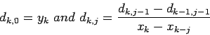
   %Use the formula above to form the divided difference table
   for j=2:n
      for k=j:n
         D(k,j)=(D(k,j-1)-D(k-1,j-1))/(X(k)-X(k-j+1));
      end
   end
   
   %Determine the coefficients of the Newton interpolatory polynomial
   C=D(n,n);
   for k=(n-1):-1:1
      C=conv(C,poly(X(k)));
      m=length(C);
      C(m)=C(m)+D(k,k);
   end
   

   Study this MATLAB code and then use the data set in the first item to
   • construct the divided-difference table by hand
   • run the MATLAB code and compare with your table
   • interpolate for $x=4$
   • extrapolate for $x=5.5$
   Solution:
   save with the name newpoly.m. Then;

   >> X=[1 2 3 5]
   >> Y=[1.06 1.12 1.34 1.78]
   >> [C,D]=newpoly(X,Y)
   C =   -0.0200    0.2000   -0.4000    1.2800
   D =
       1.0600         0         0         0
       1.1200    0.0600         0         0
       1.3400    0.2200    0.0800         0
       1.7800    0.2200         0   -0.0200
   >> C*A(4,1:4)' 
   ans =    1.7800
   >> C*[4^3 4^2 4 1]'
   ans =    1.6000
   >> C*[(5.5)^3 (5.5)^2 5.5 1]'
   ans =    1.8025