- We have mentioned that the system of normal equations for a polynomial fit is illconditioned when the degree is high. Even for a cubic least-squares polynomial, the condition number of the coefficient matrix can be large.
- In one experiment, a cubic polynomial was fitted to 21 data points. When the data were put into the coefficient matrix of Eq. 5.7, its condition number (using 2-norms) was found to be 22,000!.
- This means that small differences in the
 -values will make a large difference in the solution. In fact, if the four right-hand-side values are each changed by only 0.01 (about 0.1%), the solution for the parameters of the cubic were changed significantly, by as much as 44%!
- However, if we fit the data with orthogonal polynomials (A sequence of polynomials is said to be orthogonal with respect to the interval [a,b] if
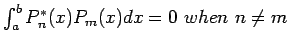 ) such as the Chebyshev polynomials. The condition number of the coefficient matrix is reduced to about 5 and the solution is not much affected by the perturbations.
Example: The following data:
R/C: 0.73, 0.78, 0.81, 0.86, 0.875, 0.89, 0.95, 1.02, l.03, 1.055, 1.135, 1.14, 1.245, 1.32, 1.385, 1.43, 1.445, 1.535, 1.57, 1.63, 1.755;
 : 0.0788, 0.0788, 0.064, 0.0788, 0.0681, 0.0703, 0.0703, 0.0681, 0.0681, 0.079, 0.0575, 0.0681, 0.0575, 0.0511, 0.0575, 0.049, 0.0532, 0.0511, 0.049, 0.0532,0.0426:
Let  and
and
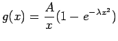
 , We would like our curve to be of the form
and our least-squares equation becomes
Setting
, We would like our curve to be of the form
and our least-squares equation becomes
Setting
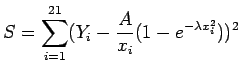
 gives the following equations:
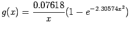
When this system of nonlinear equations is solved, we get
For these values of
gives the following equations:
When this system of nonlinear equations is solved, we get
For these values of  and
and
 . The graph of this function is presented in Figure 5.8.
Figure 5.8:
The graph of
vs  .
.
|
|
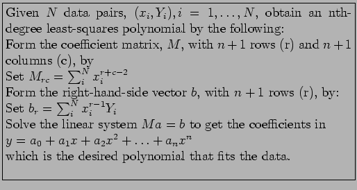
An algorithm for obtaining a least-squares polynomial:
 2004-12-28
![\includegraphics[scale=0.9]{figures/3.10.ps}](img756.png)