Least-Squares Polynomials
- Because polynomials can be readily manipulated, fitting such functions to data that do not plot linearly is common.
- It will turn out that the normal equations are linear for this situation, which is an added advantage.
 as the degree of the polynomial and N as the number of data pairs. If
  , the polynomial passes exactly through each point and the methods discussed earlier apply, so we will always have
  in the following. We assume the functional relationship
 |
(5) |
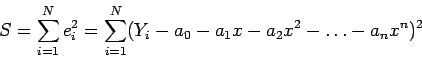
with errors defined by
We again use  to represent the observed or experimental value corresponding to
  , with free of error. We minimize the sum of squares;
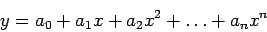
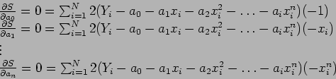
At the minimum, all the partial derivatives
 vanish. Writing the equations for these gives
  equations:
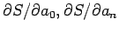
Dividing each by  and rearranging gives the normal equations to be solved simultaneously:
 |
(6) |
Putting these equations in matrix form shows the coefficient matrix;
![$\displaystyle \left[
\begin{array}{rrrrrl}
N & \sum x_i & \sum x_i^2 & \sum x_i...
...\sum x_iY_i\\
\sum x_i^2Y_i\\
\vdots \\
\sum x_i^n Y_i\\
\end{array}\right]$](img78.png) |
|
|
(7) |
All the summatins in Eqs. 6 and 7 run from 1 to  . We will let B stand for the coefficient matrix.
- Equation 7 represents a linear system. However, you need to know that this system is ill-conditioned and round-off errors can distort the solution: the
 's of Eq. 5. Up to degree-3 or -4, the problem is not too great. Special methods that use orthogonal polynomials are a remedy. Degrees higher than 4 are used very infrequently. It is often better to fit a series of lower-degree polynomials to subsets of the data.
- Matrix
 of Eq. 7 is called the normal matrix for the least-squares problem. There is another matrix that corresponds to this, called the design matrix. It is of the form;
 is just the coefficient matrix of Eq. 7. It is easy to see that
  , where
  is the column vector of
  -values, gives the right-hand side of Eq. 7. We can rewrite Eq. 7 in matrix form, as
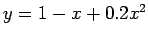
- It is illustrated the use of Eqs. 6 to fit a quadratic to the data of Table 1. Figure 7 shows a plot of the data. The data are actually a perturbation of the relation
 .
.
Table 1:
Data to illustrate curve fitting.
![\begin{table}\begin{center}
\includegraphics[scale=1]{figures/3.9.ps}
\end{center}
\end{table}](img85.png) |
Figure 7:
Figure for the data to illustrate curve fitting.
|
|
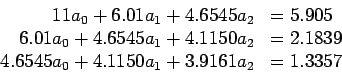
To set up the normal equations, we need the sums tabulated in Table 1. The equations to be solved are:
The result is  ,
, 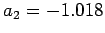 ,
, , so the least- squares method gives
which we compare to
. Errors in the data cause the equations to differ.
2004-12-06
![\begin{displaymath}
A=\left[
\begin{array}{rrrrr}
1 & 1 & 1 & 1 & 1 \\
x_1 & ...
... x_1^n & x_2^n & x_3^n & \ldots & x_N^n\\
\end{array} \right]
\end{displaymath}](img80.png)
![\includegraphics[scale=1]{figures/3.7.ps}](img86.png)