Chebyshev Series
- By rearranging the Chebyshev polynomials,
- we can express powers of
 in terms of them:
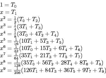 |
(6.2) |
- By substituting these identities into an infinite Taylor series
- and collecting terms in
 , we create a Chebyshev series.
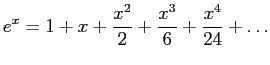
- For example, we can get the first four terms of a Chebyshev series
by starting with the Maclaurin expansion for  .
.
- Such a series converges more rapidly than does a Taylor series on
![$ [-1, 1]$](img948.png) ;
;
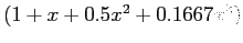
- Replacing terms by Eqn. 6.2, but omitting polynomials beyond
 because we want only four terms, we have;
- The number of terms that are employed determines the accuracy of the computed values.
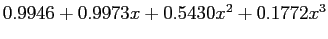
- To compare the Chebyshev expansion with the Maclaurin series, we convert back to powers of , using Eqn. 6.1:
 |
(6.3) |
Table 6.2:
Comparison of Chebyshev series for with Maclaurin series.
![\begin{table}\begin{center}
\includegraphics[scale=0.8]{figures/4.3.ps}
\end{center}
\end{table}](img953.png) |
- Table 6.2 and Figure 6.2 compare the error of the Chebyshev expansion (
 ) with the Maclaurin series
 .
.
- Chebyshev expansion, the errors can be considered to be distributed more or less uniformly throughout the interval.
- Maclaurin expansion, which gives very small errors near the origin, allows the error to bunch up at the ends of the interval.
Figure 6.2:
Comparison of the error of Chebyshev series for with the error of Maclaurin series.
|
|
Cem Ozdogan
2011-12-27
![\includegraphics[scale=1]{figures/4.4.ps}](img956.png)