List of Figures

1. MATLAB Desktop.
2. An illustrating example: The ladder in the mine.
3. An illustrating example: The ladder in the mine. Solution with MATLAB
4. Level of precision.
5. Computer numbers with six bit representation.
6. Upper: number line in the hypothetical system, Lower: IEEE standard.
7. Left: Adding eight numbers sequentially. Right: Adding eight numbers with parallel processors.
8. Testing for a change in sign of f(x) will bracket either a root or singularity.
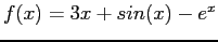
9. Plot of the function: $f(x)=3x + sin(x) - e^x$
10. The stopping criterion for a root-finding procedure should involve a tolerance on $x$, as well as a tolerance on $f(x)$.
11. Graphical illustration of the Secant Method.
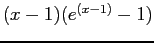
12. A pathological case for the secant method.
13. Graphical illustration of the Newton's Method.
14. Graphical illustration of the case that Newton's Method will not converge.
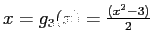
15. Parabola $a\nu ^2 + b\nu + c=p_2(\nu )$
16. An example of the use of Muller's method.
17. Cont. An example of the use of Muller's method.
18. The fixed point of $x=g(x)$ is the intersection of the line $y=x$ and the curve $y = g(x)$ plotted against $x$. Where A: $x = g_1(x) =\sqrt {2x + 3}$. B: $x=g_2(x)=\frac {3}{(x-2)}$. C: $x=g_3(x)=\frac {(x^2-3)}{2}$.
19. Left: The curve on the left has a triple root at $x = -1$ [the function is $(x + 1)^3$]. The curve on the right has a double root at $x = 2$ [the function is $(x - 2)^2$].Right: Plot of $(x - 1) (e^{(x-1)} - 1)$.
20. A pair of equations.
21. A curve fit function passes near the data points. An interpolating function passes exactly through the data points.
22. Fitting with different degrees of the polynomial.
23. Fitting with quadratic in subinterval.
24. Linear spline.
25. Cubic spline.
26. Resistance vs Temperature graph for the Least-Squares Approximation.
27. Minimizing the deviations by making the sum a minimum.
28. Figure for the data to illustrate curve fitting.
29. The graph of $V_\theta /V_\infty$ vs $R/C$.
30. plot(x,Y,'o',x,y,'-').
31. plot(x,Y,'o',x,f,'-',x,y,'+').
32. Plot of the first four polynomials of the Chebyshev polynomials.
33. Comparison of the error of Chebyshev series for $e^x$ with the error of Maclaurin series.
34. plot(x,errorchebyshev,'o',x,errormaclaurin,'-').
35. Plot of a periodic function of period P.
36. Left: Plot of $f(x)=x$, periodic of period $2\pi$,Right: Plot of the Fourier series expansion for $N=2,4,8$.
37. Plot of Fourier series for $\vert x\vert$ for $N=2,4,8$.
38. Plot of Fourier series for $x(2-x)$ for $N=40$.
39. A function, $f(x)$, of interest on [0,3].
40. Left: Plot of a function reflected about the y-axis, an even function,Right: Plot of a function reflected about the origin, an odd function.
41. Left: Plot of the function reflected about the y-axis, Right: Plot of the function reflected about the origin.
42. The trapezoidal rule.